-
Python 데이터분석 기초 38 - 어느 음식점 매출 자료와 날씨 자료를 활용하여 온도(추움, 보통, 더움)에 따른 매출액 평균에 차이를 검정 + 웹Python 데이터 분석 2022. 11. 9. 13:12
# 어느 음식점 매출 자료와 날씨 자료를 활용하여 온도(추움, 보통, 더움)에 따른 매출액 평균에 차이를 검정

# 귀무 : 음식점 매출액의 평균은 온도에 영향이 없다.
# 대립 : 음식점 매출액의 평균은 온도에 영향이 있다.

import numpy as np
import scipy.stats as stats
import pandas as pd
import matplotlib.pyplot as plt

# 데이터는 data.go.kr을 참조
# 매출 자료
sales_data = pd.read_csv("https://raw.githubusercontent.com/pykwon/python/master/testdata_utf8/tsales.csv", dtype={'YMD':'object'}) # 데이터 타입 바꾸기
print(sales_data.head(3))
print(sales_data.info()) # 328 * 3

# 날씨 자료
wt_data = pd.read_csv("https://raw.githubusercontent.com/pykwon/python/master/testdata_utf8/tweather.csv")
print(wt_data.head(3))
print(wt_data.info()) # 702 * 9

# 두 데이터를 병합 : 날짜를 사용.  그래서 wt_data의 tm을 2018-06-01 ==> 20180601 형태로 변환
wt_data.tm = wt_data.tm.map(lambda x:x.replace('-','')) # 데이터를 하나만 꺼냈기 때문에 시리즈 데이터이다. 그래서 map함수 사용
print(wt_data.head(3))
print(wt_data.tail(3))

print('merge --------')
frame = sales_data.merge(wt_data, how = 'left', left_on = 'YMD', right_on = 'tm')
print(frame.head(5))
print(frame.tail(5))
print(len(frame))   # 328행

print()
# 분석에 사용할 열만 추출
print(frame.columns) # ['YMD', 'AMT', 'CNT', 'stnId', 'tm', 'avgTa', 'minTa', 'maxTa', 'sumRn', 'maxWs', 'avgWs', 'ddMes']
data = frame.iloc[:, [0, 1, 7, 8]] # 'YMD', 'AMT' 'maxTa', 'sumRn'
print(data.head(3))

# 일별 최고온도(maxTa)를 구간설정을 해서 범주형 변수를 추가
print(data.maxTa.describe())

data['Ta_gubun'] = pd.cut(data.maxTa, bins = [-5, 8, 24, 37], labels = [0,1,2]) # 3개의 구간으로 나눴다.
print(data.isnull().sum()) # 결측치 확인
print(data['Ta_gubun'].unique()) # 어떤 값이 있는지 호출

# 세 그룹의 매출액으로 정규성, 등분산성 확인
x1 = np.array(data[data.Ta_gubun == 0].AMT)
x2 = np.array(data[data.Ta_gubun == 1].AMT)
x3 = np.array(data[data.Ta_gubun == 2].AMT)
print(x1[:5])
print(x2[:5])
print(x3[:5])

# 정규성
print(stats.ks_2samp(x1, x2).pvalue) # 만족 못함
print(stats.ks_2samp(x1, x3).pvalue) # 만족 못함
print(stats.ks_2samp(x2, x3).pvalue) # 만족 못함

# 등분산성
print(stats.levene(x1, x2, x3).pvalue) # 표본수가 클 때 사용하는 levene 사용. 0.0390023 < 0.05 만족 못함

print('온도별 매출액 평균')
# pd.options.display.float_format = '{:.5f}'.format  # 과학적 표기법 해제
spp = data.loc[:,['AMT','Ta_gubun']]
print(spp.head(2))
print(spp.groupby('Ta_gubun').mean())

print(pd.pivot_table(spp, index = ['Ta_gubun'], aggfunc = 'mean')) # groupby 함수와 같은 방법
# 1032362 vs 818106 vs 553710 차이?

# anova 진행
sp = np.array(spp) # DataFrame을 np.array로 바꾸기
print(sp[:3])
group1 = sp[sp[:, 1] == 0, 0] # 1열이 0인 거의 0번째 열
group2 = sp[sp[:, 1] == 1, 0]
group3 = sp[sp[:, 1] == 2, 0]

# 데이터 분포 시각화
# plt.boxplot([group1, group2, group3], showmeans = True)
# plt.show()

print() # 요인이 하나 데이터가 여러개일때 사용
print(stats.f_oneway(group1, group2, group3))
# statistic=99.1908012029983, pvalue=2.360737101089604e-34
# 해석 : pvalue=2.360737101089604e-34 < 0.05 이므로 귀무 기각.
# 음식점 매출액의 평균은 온도에 영향이 있다.

# 정규성을 만족하지 않으므로
print(stats.kruskal(group1, group2, group3))
# KruskalResult(statistic=132.7022591443371, pvalue=1.5278142583114522e-29)
# 여전히 기각

# 등분산성을 마족하지 않으므로
# pip install pingouin
from pingouin import welch_anova
print(welch_anova(data=data, dv='AMT', between='Ta_gubun'))
#      Source  ddof1     ddof2           F         p-unc       np2
# 0  Ta_gubun      2  189.6514  122.221242  7.907874e-35  0.379038
# 여전히 기각


# 각 매출액의 평균차이가 궁금. 사후검정 수행
# post hoc test
from statsmodels.stats.multicomp import pairwise_tukeyhsd
turkeyResult = pairwise_tukeyhsd(endog = spp.AMT, groups = spp.Ta_gubun, alpha = 0.05)
print(turkeyResult)  # 차이가 없으면 reject가 False가 나오고, 차이가 크면 True가 나온다.

# 시각화
turkeyResult.plot_simultaneous(xlabel = 'mean', ylabel = 'group')
plt.show()


<console>
        YMD    AMT  CNT
0  20190514      0    1
1  20190519  18000    1
2  20190521  50000    4
<class 'pandas.core.frame.DataFrame'>
RangeIndex: 328 entries, 0 to 327
Data columns (total 3 columns):
 #   Column  Non-Null Count  Dtype
---  ------  --------------  -----
 0   YMD     328 non-null    object
 1   AMT     328 non-null    int64
 2   CNT     328 non-null    int64
dtypes: int64(2), object(1)
memory usage: 7.8+ KB
None
   stnId          tm  avgTa  minTa  maxTa  sumRn  maxWs  avgWs  ddMes
0    108  2018-06-01   23.8   17.5   30.2    0.0    4.3    1.9    0.0
1    108  2018-06-02   23.4   17.6   30.1    0.0    4.5    2.0    0.0
2    108  2018-06-03   24.0   16.9   30.8    0.0    4.2    1.6    0.0
<class 'pandas.core.frame.DataFrame'>
RangeIndex: 702 entries, 0 to 701
Data columns (total 9 columns):
 #   Column  Non-Null Count  Dtype
---  ------  --------------  -----
 0   stnId   702 non-null    int64
 1   tm      702 non-null    object
 2   avgTa   702 non-null    float64
 3   minTa   702 non-null    float64
 4   maxTa   702 non-null    float64
 5   sumRn   702 non-null    float64
 6   maxWs   702 non-null    float64
 7   avgWs   702 non-null    float64
 8   ddMes   702 non-null    float64
dtypes: float64(7), int64(1), object(1)
memory usage: 49.5+ KB
None
   stnId        tm  avgTa  minTa  maxTa  sumRn  maxWs  avgWs  ddMes
0    108  20180601   23.8   17.5   30.2    0.0    4.3    1.9    0.0
1    108  20180602   23.4   17.6   30.1    0.0    4.5    2.0    0.0
2    108  20180603   24.0   16.9   30.8    0.0    4.2    1.6    0.0
     stnId        tm  avgTa  minTa  maxTa  sumRn  maxWs  avgWs  ddMes
699    108  20200430   17.1    9.3   23.4    0.0    5.9    2.7    0.0
700    108  20200501   20.2   16.4   26.2    0.0    5.5    2.7    0.0
701    108  20200502   20.3   18.0   23.9    0.0    4.6    2.3    0.0
merge --------
        YMD     AMT  CNT  stnId        tm  ...  maxTa  sumRn  maxWs  avgWs  ddMes
0  20190514       0    1    108  20190514  ...   26.9    0.0    4.1    1.6    0.0
1  20190519   18000    1    108  20190519  ...   21.6   22.0    2.7    1.2    0.0
2  20190521   50000    4    108  20190521  ...   23.8    0.0    5.9    2.9    0.0
3  20190522  125000    7    108  20190522  ...   26.5    0.0    5.4    2.4    0.0
4  20190523  222500   13    108  20190523  ...   29.2    0.0    3.5    1.7    0.0

[5 rows x 12 columns]
          YMD      AMT  CNT  stnId        tm  ...  maxTa  sumRn  maxWs  avgWs  ddMes
323  20200424  1092500   51    108  20200424  ...   14.3    0.0    8.2    3.9    0.0
324  20200425   672500   34    108  20200425  ...   17.1    0.0    7.8    3.9    0.0
325  20200426  1123500   55    108  20200426  ...   19.0    0.0    6.5    3.2    0.0
326  20200427   819500   45    108  20200427  ...   18.3    0.0    5.5    2.8    0.0
327  20200428   950500   45    108  20200428  ...   19.9    0.0    5.5    3.0    0.0

[5 rows x 12 columns]
328

Index(['YMD', 'AMT', 'CNT', 'stnId', 'tm', 'avgTa', 'minTa', 'maxTa', 'sumRn',
       'maxWs', 'avgWs', 'ddMes'],
      dtype='object')
        YMD    AMT  maxTa  sumRn
0  20190514      0   26.9    0.0
1  20190519  18000   21.6   22.0
2  20190521  50000   23.8    0.0
count    328.000000
mean      18.597866
std       10.163039
min       -4.900000
25%        9.375000
50%       19.350000
75%       27.800000
max       36.800000
Name: maxTa, dtype: float64
C:\Users\JEONGYEON\Desktop\Python\Python\pro1\pack8anal2\anova3.py:42: SettingWithCopyWarning:
A value is trying to be set on a copy of a slice from a DataFrame.
Try using .loc[row_indexer,col_indexer] = value instead

See the caveats in the documentation: https://pandas.pydata.org/pandas-docs/stable/user_guide/indexing.html#returning-a-view-versus-a-copy
  data['Ta_gubun'] = pd.cut(data.maxTa, bins = [-5, 8, 24, 37], labels = [0,1,2]) # 3개의 구간으로 나눴다.
YMD         0
AMT         0
maxTa       0
sumRn       0
Ta_gubun    0
dtype: int64
[2, 1, 0]
Categories (3, int64): [0 < 1 < 2]
[1050500  770000 1054500  969000 1061500]
[ 18000  50000 274000 203000 381500]
[     0 125000 222500 209000 302000]
9.28938415079017e-09
1.198570472122961e-28
1.4133139103478243e-13
0.039002396565063324
온도별 매출액 평균
     AMT Ta_gubun
0      0        2
1  18000        1
                   AMT
Ta_gubun
0         1.032362e+06
1         8.181069e+05
2         5.537109e+05
                   AMT
Ta_gubun
0         1.032362e+06
1         8.181069e+05
2         5.537109e+05
[[    0     2]
 [18000     1]
 [50000     1]]

F_onewayResult(statistic=99.1908012029983, pvalue=2.360737101089604e-34)
KruskalResult(statistic=132.7022591443371, pvalue=1.5278142583114522e-29)
     Source  ddof1     ddof2           F         p-unc       np2
0  Ta_gubun      2  189.6514  122.221242  7.907874e-35  0.379038
       Multiple Comparison of Means - Tukey HSD, FWER=0.05
=================================================================
group1 group2   meandiff   p-adj    lower        upper     reject
-----------------------------------------------------------------
     0      1 -214255.4486   0.0  -296755.647 -131755.2503   True
     0      2 -478651.3813  -0.0 -561484.4539 -395818.3088   True
     1      2 -264395.9327  -0.0 -333326.1167 -195465.7488   True
-----------------------------------------------------------------
정규성, 등분산성을 만족하지 못 할때 사용할 함수도 내용에 들어있다.

데이터 분포 시각화 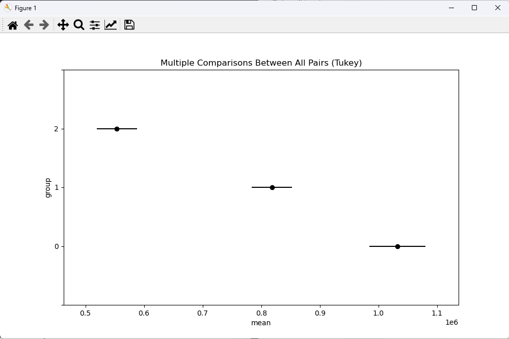
사후검정 시각화 'Python 데이터 분석' 카테고리의 다른 글
Python 데이터분석 기초 39 - Two-way ANOVA(이원분산분석) (0) 2022.11.09 ANOVA 예제 1, 2(정규성, 등분산성 검정, 사후 검정) 귀무 vs 대립 (1) 2022.11.09 Python 데이터분석 기초 37 - 일원분산분석으로 평균차이 검정(웹에서 데이터 가져오기) (0) 2022.11.09 Python 데이터분석 기초 36 - 세 개 이상의 모집단에 대한 가설검정 – 분산분석(ANOVA), 사후검정 (0) 2022.11.09 t-test 검정 문제(2) DB 예제, 정규성 확인 (0) 2022.11.08