-
단순선형회귀 방법 1, 방법 2 예제(Sequential api, Function api)TensorFlow 2022. 11. 30. 15:31

방법1
import tensorflow as tf
from keras.models import Sequential
from keras.layers import Dense, Activation
from keras import optimizers
import numpy as np
import pandas as pd
from sklearn.model_selection import train_test_split
from sklearn.metrics import r2_score
from keras.optimizers import SGD, RMSprop, Adam

df = pd.read_table('http://www.randomservices.org/random/data/Galton.txt')
df = df.loc[(df['Gender'] == 'M')].drop('Gender', axis=1)
print(df.head(3))

x = df['Father']
y = df['Height']
print(x[:3])
print(y[:3])
print(np.corrcoef(x, y)) # 0.391

# train / test split (7 : 3)
x_train, x_test, y_train, y_test = train_test_split(x, y, test_size = 0.3, random_state = 0)
print(x_train.shape, x_test.shape, y_train.shape, y_test.shape) # (325,) (140,) (325,) (140,)

model = Sequential()
model.add(Dense(units=5, input_dim=1, activation='linear'))
model.add(Dense(units=1, activation='linear'))
print(model.summary())

opti = optimizers.Adam(learning_rate=0.01)
model.compile(optimizer=opti, loss='mse', metrics=['mse'])

history = model.fit(x_train, y_train, batch_size=4, epochs=100, verbose=0)
loss_metrics = model.evaluate(x_test, y_test, verbose=0)
print('loss_metrics :', loss_metrics)

print('설명력 :', r2_score(y_test, model.predict(x_test)))
print('실제값 :', y_test[:5].values)
print('예측값 :', model.predict(x_test).flatten()[:5])

# 새로운 값 예측
new_height = [75, 70, 80]
print('새로운 예측값: ', model.predict(new_height).flatten())

# 시각화
import matplotlib.pyplot as plt
plt.rc('font', family='malgun gothic')
plt.plot(x_train, model.predict(x_train), 'b', x_test, y_test, 'ko') # train
plt.show()

plt.plot(x_test, model.predict(x_test), 'b', x_test, y_test, 'ko')  # test
plt.show()

plt.plot(history.history['mse'], label='평균제곱오차')
plt.xlabel('학습 횟수')
plt.show()


<console>
  Family  Father  Mother  Height  Kids
0      1    78.5    67.0    73.2     4
4      2    75.5    66.5    73.5     4
5      2    75.5    66.5    72.5     4
0    78.5
4    75.5
5    75.5
Name: Father, dtype: float64
0    73.2
4    73.5
5    72.5
Name: Height, dtype: float64
[[1.         0.39131736]
 [0.39131736 1.        ]]
(325,) (140,) (325,) (140,)
Model: "sequential"
_________________________________________________________________
 Layer (type)                Output Shape              Param #
=================================================================
 dense (Dense)               (None, 5)                 10

 dense_1 (Dense)             (None, 1)                 6

=================================================================
Total params: 16
Trainable params: 16
Non-trainable params: 0
_________________________________________________________________
None
loss_metrics : [13.743265151977539, 13.743265151977539]

1/5 [=====>........................] - ETA: 0s
5/5 [==============================] - 0s 500us/step
설명력 : -1.0972842836983117
실제값 : [68.  67.  70.  67.  70.2]

1/5 [=====>........................] - ETA: 0s
5/5 [==============================] - 0s 997us/step
예측값 : [67.28584  70.39301  72.14079  73.111786 69.22783 ]

1/1 [==============================] - ETA: 0s
1/1 [==============================] - 0s 53ms/step
새로운 예측값:  [76.99574 72.14079 81.85071]

 1/11 [=>............................] - ETA: 0s
11/11 [==============================] - 0s 708us/step

1/5 [=====>........................] - ETA: 0s
5/5 [==============================] - 0s 748us/step
방법2
print('\n--Function api 사용------------------------------')
from keras.layers import Input
from keras.models import Model

inputs = Input(shape=(1,))
output1 = Dense(units=5, activation='linear')(inputs)
outputs = Dense(1, activation='linear')(output1)

model2 = Model(inputs, outputs)
print(model2.summary())

opti = tf.keras.optimizers.Adam(learning_rate=0.001)
model2.compile(optimizer=opti, loss='mse', metrics=['mse'])
history = model2.fit(x=x_train, y=y_train, epochs=50, batch_size=4, verbose=0)
loss_metrics2 = model2.evaluate(x=x_test, y=y_test, verbose=0)
print('loss metrics: ', loss_metrics2)
print('실제값 : ', y_test.head().values)
print('예측값 :', model2.predict(x_test).flatten()[:5])
print()

new_data = [75, 70, 80]
print('새로운 예측 키 값: ', model2.predict(new_data).flatten())


<console>
--Function api 사용------------------------------
Model: "model"
_________________________________________________________________
 Layer (type)                Output Shape              Param #
=================================================================
 input_1 (InputLayer)        [(None, 1)]               0

 dense_2 (Dense)             (None, 5)                 10

 dense_3 (Dense)             (None, 1)                 6

=================================================================
Total params: 16
Trainable params: 16
Non-trainable params: 0
_________________________________________________________________
None
loss metrics:  [8.111572265625, 8.111572265625]
실제값 :  [68.  67.  70.  67.  70.2]

1/5 [=====>........................] - ETA: 0s
5/5 [==============================] - 0s 748us/step
예측값 : [65.24897  68.451355 70.2527   71.25345  67.25046 ]


1/1 [==============================] - ETA: 0s
1/1 [==============================] - 0s 50ms/step
새로운 예측 키 값:  [75.25643 70.2527  80.26017]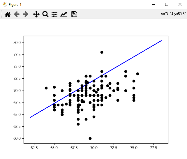
train 시각화 
test 시각화 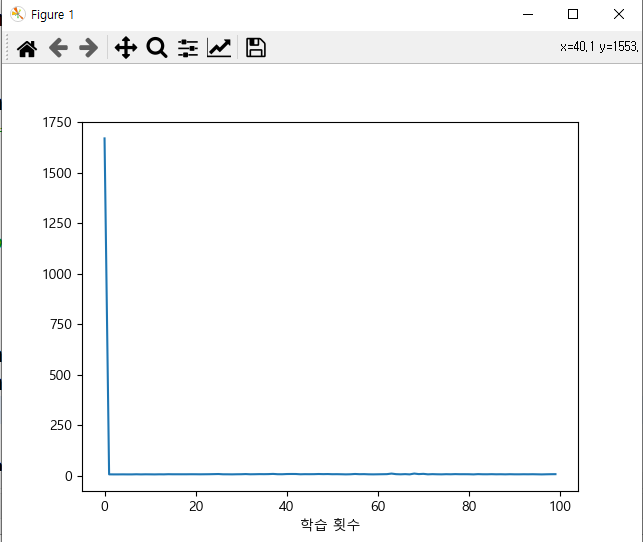
'TensorFlow' 카테고리의 다른 글
TensorFlow 기초 13 - 다중선형회귀모델(scaling) - 정규화, 표준화 validation_split (0) 2022.11.30 TensorFlow 기초 12 - 다중선형회귀모델 작성 후 텐서보드(모델의 구조 및 학습과정/결과를 시각화) - (0) 2022.11.30 TensorFlow 기초 11 - 단순선형회귀모델 작성 : 방법 3가지(다중 입출력 모델) (0) 2022.11.30 TensorFlow 기초 10 - 선형회귀분석 예제(예측, 결정계수) (0) 2022.11.30 TensorFlow 기초 9 - 선형회귀 모형 작성 = 수식 사용(Keras 없이 tensorflow만 사용) - GradientTape (0) 2022.11.29