Python 데이터분석 기초 63 - DecisionTreeRegressor, RandomForestRegressor

 

중요변수 얻을 때는 RandomForestRegressor를 사용하는 것을 추천한다.

그 이외에는 ols를 추천

 

#

import pandas as pd
import matplotlib.pyplot as plt
import seaborn as sns
from sklearn.tree import DecisionTreeRegressor
from sklearn.ensemble import RandomForestRegressor
from sklearn.datasets import load_boston
from sklearn.metrics import r2_score

boston = load_boston()
# print(boston.keys())

dfx = pd.DataFrame(boston.data, columns = boston.feature_names)
dfy = pd.DataFrame(boston.target, columns = ['MEDV'])
df = pd.concat([dfx, dfy], axis = 1)
print(df.head(3))
print(df.corr())

# 시각화
cols = ['MEDV', 'RM', 'LSTAT']
# sns.pairplot(df[cols])
# plt.show()

# 단순선형회귀
x = df[['LSTAT']].values
y = df['MEDV'].values
print(x[:3])
print(y[:3])

print('DecisionTreeRegressor')
model = DecisionTreeRegressor(criterion = 'mse', random_state = 123).fit(x, y)
print('예측값 :', model.predict(x[:5]))
print('실제값 :', y[:5])
print('결정계수 :', r2_score(y, model.predict(x))) # 0.9590

print('RandomForestRegressor')
model2 = RandomForestRegressor(criterion = 'mse', n_estimators = 100, random_state = 123).fit(x, y)
print('예측값 :', model2.predict(x[:5]))
print('실제값 :', y[:5])
print('결정계수 :', r2_score(y, model2.predict(x))) # 0.9081



<console>
      CRIM    ZN  INDUS  CHAS    NOX  ...    TAX  PTRATIO       B  LSTAT  MEDV
0  0.00632  18.0   2.31   0.0  0.538  ...  296.0     15.3  396.90   4.98  24.0
1  0.02731   0.0   7.07   0.0  0.469  ...  242.0     17.8  396.90   9.14  21.6
2  0.02729   0.0   7.07   0.0  0.469  ...  242.0     17.8  392.83   4.03  34.7

[3 rows x 14 columns]
             CRIM        ZN     INDUS  ...         B     LSTAT      MEDV
CRIM     1.000000 -0.200469  0.406583  ... -0.385064  0.455621 -0.388305
ZN      -0.200469  1.000000 -0.533828  ...  0.175520 -0.412995  0.360445
INDUS    0.406583 -0.533828  1.000000  ... -0.356977  0.603800 -0.483725
CHAS    -0.055892 -0.042697  0.062938  ...  0.048788 -0.053929  0.175260
NOX      0.420972 -0.516604  0.763651  ... -0.380051  0.590879 -0.427321
RM      -0.219247  0.311991 -0.391676  ...  0.128069 -0.613808  0.695360
AGE      0.352734 -0.569537  0.644779  ... -0.273534  0.602339 -0.376955
DIS     -0.379670  0.664408 -0.708027  ...  0.291512 -0.496996  0.249929
RAD      0.625505 -0.311948  0.595129  ... -0.444413  0.488676 -0.381626
TAX      0.582764 -0.314563  0.720760  ... -0.441808  0.543993 -0.468536
PTRATIO  0.289946 -0.391679  0.383248  ... -0.177383  0.374044 -0.507787
B       -0.385064  0.175520 -0.356977  ...  1.000000 -0.366087  0.333461
LSTAT    0.455621 -0.412995  0.603800  ... -0.366087  1.000000 -0.737663
MEDV    -0.388305  0.360445 -0.483725  ...  0.333461 -0.737663  1.000000

[14 rows x 14 columns]
[[4.98]
 [9.14]
 [4.03]]
[24.  21.6 34.7]
DecisionTreeRegressor

예측값 : [24.  21.6 34.7 33.4 32.8]
실제값 : [24.  21.6 34.7 33.4 36.2]
결정계수 : 0.9590088126871839
RandomForestRegressor

예측값 : [24.469      21.975      35.48173333 38.808      32.11911667]
실제값 : [24.  21.6 34.7 33.4 36.2]
결정계수 : 0.9081654854048482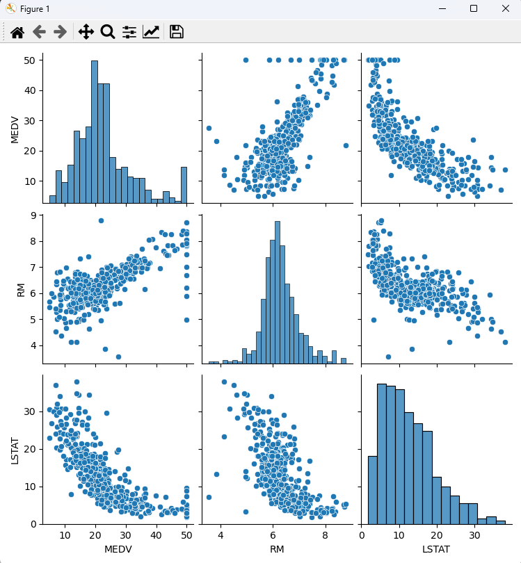

 

 

MEDV, RM, LSTAT 관계 시각화