회귀분석모형의 적절성을 위한 5가지 조건 예제

 

 

# 회귀분석 문제 3) 
# kaggle.com에서 carseats.csv 파일을 다운 받아 (https://github.com/pykwon 에도 있음)
# Sales 변수에 영향을 주는 변수들을 선택하여 선형회귀분석을 실시한다.
# 변수 선택은 모델.summary() 함수를 활용하여 타당한 변수만 임의적으로 선택한다.
# 회귀분석모형의 적절성을 위한 조건도 체크하시오.
# 완성된 모델로 Sales를 예측.

import numpy as np
import pandas as pd
import matplotlib.pyplot as plt
import statsmodels.api
plt.rc('font', family = 'malgun gothic')
import seaborn as sns
import statsmodels.formula.api as smf

df = pd.read_csv('../testdata/Carseats.csv')
print(df.head(2))
print(df.info())
df = df.drop([df.columns[6], df.columns[9], df.columns[10]], axis = 1) # 6, 9, 10 열은 제외.
print(df.head(2))
print(df.corr()) # 상관관계 확인
lm = smf.ols(formula = 'Sales ~ Income + Advertising + Price + Age', data = df).fit()
print('요약 결과: \n', lm.summary()) # p-value : 1.33e-38 < 0.05 이므로 유의한 데이터이다.

df_lm = df.iloc[:,[0, 2, 3, 5, 6]]
print(df_lm)


print('---회귀분석모형의 적절성 확인 작업')
# 잔차 구하기
fitted = lm.predict(df_lm) # 예측값
residual = df_lm['Sales'] - fitted # 실제값 - 예측값
print(residual[:3])
print('잔차의 평균 :', np.mean(residual)) # -8.057998712729386e-15

print('--- 선형성 ---')
sns.regplot(fitted, residual, lowess = True, line_kws = {'color':'red'})
plt.plot([fitted.min(), fitted.max()], [0, 0], '--', c = 'b')
plt.show() # 잔차가 일정하게 분포되어 있으므로 선형성 만족

print('--- 정규성 ---')
import scipy.stats as stats
sr = stats.zscore(residual)
(x, y), _ = stats.probplot(sr)
sns.scatterplot(x, y)
plt.plot([-3, 3], [-3, 3], '--', c = 'b')
plt.show() # 잔차항이 정규분포를 따름

print('shapiro test :', stats.shapiro(residual)) # p-value : 0.2127407342195511 > 0.05 이므로 정규성 만족

print('--- 독립성 ---')
# Durbin-Watson : 1.931   2에 근사하므로 독립성 만족

print('--- 등분산성 ---')
sr = stats.zscore(residual)
sns.regplot(fitted, np.sqrt(abs(sr)), lowess = True, line_kws = {'color':'red'})
plt.show() # 평균선을 기준으로 일정한 패턴을 보이지 않아 등분산성 만족.

print('--- 다중공선성 ---')
from statsmodels.stats.outliers_influence import variance_inflation_factor
df2 = df[['Income', 'Advertising', 'Price', 'Age']]
print(df2.head(2))
print(df2.shape) # (400, 4)
vifdf = pd.DataFrame()
vifdf['vif_value'] = [variance_inflation_factor(df2.values, i) for i in range(df2.shape[1])]
print(vifdf) # 모든 변수가 10을 넘기지 않음. 다중공선성 우려 없음.


# 모델 저장
import joblib
joblib.dump(lm, 'yhs.model') # yhs.model 이름으로 저장
del lm # 이 페이지에서 삭제
print('-----지금부터는 저장된 모델을 읽어 사용함------')
lm = joblib.load('yhs.model')
# print(lm_dajung.summary())


# 완성된 모델로 새로운 독립변수의 값을 주고 Sales를 예측
new_df = pd.DataFrame({'Income':[33, 55, 66], 'Advertising':[10, 13, 16],
                       'Price':[100, 120, 140], 'Age':[33, 35, 40]})
pred = lm.predict(new_df)
print('Sales에 대한 예측 결과 : \n', pred)


<console>
   Sales  CompPrice  Income  Advertising  ...  Age  Education Urban   US
0   9.50        138      73           11  ...   42         17   Yes  Yes
1  11.22        111      48           16  ...   65         10   Yes  Yes

[2 rows x 11 columns]
<class 'pandas.core.frame.DataFrame'>
RangeIndex: 400 entries, 0 to 399
Data columns (total 11 columns):
 #   Column       Non-Null Count  Dtype  
---  ------       --------------  -----  
 0   Sales        400 non-null    float64
 1   CompPrice    400 non-null    int64  
 2   Income       400 non-null    int64  
 3   Advertising  400 non-null    int64  
 4   Population   400 non-null    int64  
 5   Price        400 non-null    int64  
 6   ShelveLoc    400 non-null    object 
 7   Age          400 non-null    int64  
 8   Education    400 non-null    int64  
 9   Urban        400 non-null    object 
 10  US           400 non-null    object 
dtypes: float64(1), int64(7), object(3)
memory usage: 34.5+ KB
None
   Sales  CompPrice  Income  Advertising  Population  Price  Age  Education
0   9.50        138      73           11         276    120   42         17
1  11.22        111      48           16         260     83   65         10
                Sales  CompPrice    Income  ...     Price       Age  Education
Sales        1.000000   0.064079  0.151951  ... -0.444951 -0.231815  -0.051955
CompPrice    0.064079   1.000000 -0.080653  ...  0.584848 -0.100239   0.025197
Income       0.151951  -0.080653  1.000000  ... -0.056698 -0.004670  -0.056855
Advertising  0.269507  -0.024199  0.058995  ...  0.044537 -0.004557  -0.033594
Population   0.050471  -0.094707 -0.007877  ... -0.012144 -0.042663  -0.106378
Price       -0.444951   0.584848 -0.056698  ...  1.000000 -0.102177   0.011747
Age         -0.231815  -0.100239 -0.004670  ... -0.102177  1.000000   0.006488
Education   -0.051955   0.025197 -0.056855  ...  0.011747  0.006488   1.000000

[8 rows x 8 columns]
요약 결과: 
                             OLS Regression Results                            
==============================================================================
Dep. Variable:                  Sales   R-squared:                       0.371
Model:                            OLS   Adj. R-squared:                  0.364
Method:                 Least Squares   F-statistic:                     58.21
Date:                Wed, 16 Nov 2022   Prob (F-statistic):           1.33e-38
Time:                        12:27:19   Log-Likelihood:                -889.67
No. Observations:                 400   AIC:                             1789.
Df Residuals:                     395   BIC:                             1809.
Df Model:                           4                                         
Covariance Type:            nonrobust                                         
===============================================================================
                  coef    std err          t      P>|t|      [0.025      0.975]
-------------------------------------------------------------------------------
Intercept      15.1829      0.777     19.542      0.000      13.656      16.710
Income          0.0108      0.004      2.664      0.008       0.003       0.019
Advertising     0.1203      0.017      7.078      0.000       0.087       0.154
Price          -0.0573      0.005    -11.932      0.000      -0.067      -0.048
Age            -0.0486      0.007     -6.956      0.000      -0.062      -0.035
==============================================================================
Omnibus:                        3.285   Durbin-Watson:                   1.931
Prob(Omnibus):                  0.194   Jarque-Bera (JB):                3.336
Skew:                           0.218   Prob(JB):                        0.189
Kurtosis:                       2.903   Cond. No.                     1.01e+03
==============================================================================

     Sales  Income  Advertising  Price  Age
0     9.50      73           11    120   42
1    11.22      48           16     83   65
2    10.06      35           10     80   59
3     7.40     100            4     97   55
4     4.15      64            3    128   38
..     ...     ...          ...    ...  ...
395  12.57     108           17    128   33
396   6.14      23            3    120   55
397   7.41      26           12    159   40
398   5.94      79            7     95   50
399   9.71      37            0    120   49

[400 rows x 5 columns]
---회귀분석모형의 적절성 확인 작업
0    1.121679
1    1.509747
2    0.747950
dtype: float64
잔차의 평균 : -8.057998712729386e-15
--- 선형성 ---
--- 정규성 ---
shapiro test : ShapiroResult(statistic=0.994922399520874, pvalue=0.2127407342195511)
--- 독립성 ---
--- 등분산성 ---
--- 다중공선성 ---
   Income  Advertising  Price  Age
0      73           11    120   42
1      48           16     83   65
(400, 4)
   vif_value
0   5.971040
1   1.993726
2   9.979281
3   8.267760
-----지금부터는 저장된 모델을 읽어 사용함------
Sales에 대한 예측 결과 : 
 0    9.410249
1    8.765653
2    7.856649
dtype: float64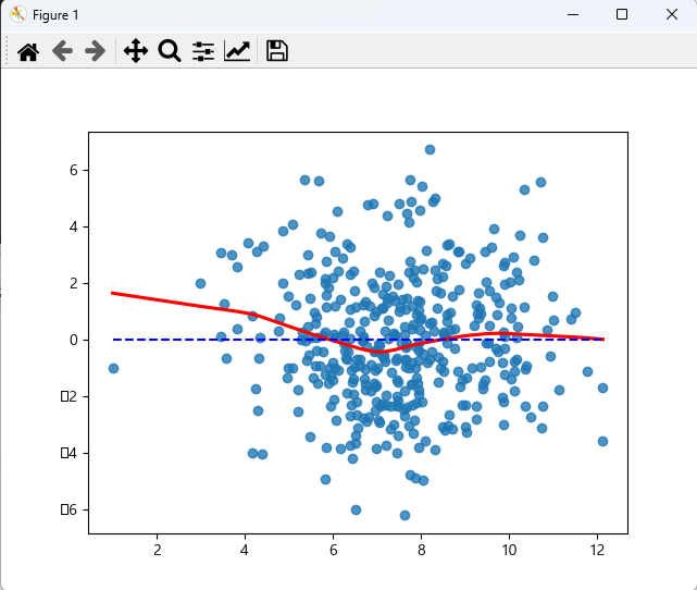

 

 

잔차 선형성 검사 시각화

잔차가 일정하게 분포되어 있으므로 선형성 만족

 

 

잔차항 정규성 검사 시각화

잔차항이 정규분포를 따르므로 정규성 만족

 

 

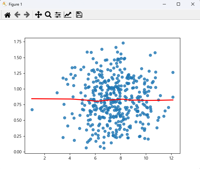
잔차항 등분산성 검사 시각화

 

모든 변수가 10을 넘기지 않으므로 다중공선성 우려 없다. 등분산성 만족