TensorFlow
TensorFlow 기초 23 - iris dataset 분류 모델 여러개 생성 후 성능 비교. 최종 모델 ROC curve 표현(모델 = 함수 사용)
코딩탕탕
2022. 12. 6. 12:28
# iris dataset 분류 모델 여러개 생성 후 성능 비교. 최종 모델 ROC curve 표현
import numpy as np
import matplotlib.pyplot as plt
from sklearn.datasets import load_iris
from sklearn.model_selection import train_test_split
from sklearn.preprocessing import OneHotEncoder, StandardScaler
iris = load_iris()
print(iris.keys())
x = iris.data
print(x[:2])
y = iris.target
print(y[:2])
names = iris.target_names # 꽃의 종류명
print(names) # ['setosa' 'versicolor' 'virginica']
feature_names = iris.feature_names
print(feature_names) # ['sepal length (cm)', 'sepal width (cm)', 'petal length (cm)', 'petal width (cm)']
# label에 대해 원핫 인코딩
print(y[:1], y.shape) # [0] (150,)
onehot = OneHotEncoder(categories='auto') # keras : to_categorical, numpy : eye(), pandas : get_dummies()
y = onehot.fit_transform(y[:, np.newaxis]).toarray()
print(y[:1], y.shape) # [[1. 0. 0.]] (150, 3)
# feature에 대해 표준화
scaler = StandardScaler()
x_scaler = scaler.fit_transform(x)
print(x_scaler[:2])
# train / test split
x_train, x_test, y_train, y_test = train_test_split(x_scaler, y, test_size=0.3, random_state=1)
n_features = x_train.shape[1]
n_classes = y_train.shape[1]
print('feature 수 : {}, label 수 : {}'.format(n_features, n_classes))
print('model')
from keras.models import Sequential
from keras.layers import Dense
def create_model_func(input_dim, output_dim, out_nodes, n, model_name='model'): # parameter 값에 초기값을 줄 수 있다.
# print(input_dim, output_dim, out_nodes, n, model_name)
def create_model():
model = Sequential(name=model_name)
for _ in range(n):
model.add(Dense(units=out_nodes, input_dim=input_dim, activation='relu'))
model.add(Dense(units=output_dim, activation='softmax')) # 출력층
model.compile(optimizer='adam', loss='categorical_crossentropy', metrics=['acc'])
return model
return create_model
models = [create_model_func(n_features, n_classes, 10, n, 'model_{}'.format(n)) for n in range(1, 4)]
print(len(models))
for cre_model in models:
print()
cre_model().summary()
history_dict = {}
for cre_model in models:
model = cre_model()
print('모델명 :', model.name)
historis = model.fit(x_train, y_train, batch_size=5, epochs=50, validation_split=0.3, verbose=0)
score = model.evaluate(x_test, y_test, verbose=0)
print('test loss :', score[0])
print('test acc :', score[1])
history_dict[model.name] = [historis, model]
print(history_dict)
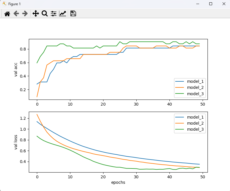
# 모델 성능 확인을 위한 시각화
fig, (ax1, ax2) = plt.subplots(2, 1, figsize=(8, 6))
for model_name in history_dict:
print('h_d :', history_dict[model_name][0].history['acc'])
val_acc = history_dict[model_name][0].history['val_acc']
val_loss = history_dict[model_name][0].history['val_loss']
ax1.plot(val_acc, label=model_name)
ax2.plot(val_loss, label=model_name)
ax1.set_ylabel('val acc')
ax2.set_ylabel('val loss')
ax2.set_ylabel('val loss')
ax2.set_xlabel('epochs')
ax1.legend()
ax2.legend()
plt.show()
# ROC curve로 모델 성능 확인
from sklearn.metrics import roc_curve, auc
plt.figure()
plt.plot([0, 1], [0, 1], 'k--')
for model_name in history_dict:
model = history_dict[model_name][1]
y_pred = model.predict(x_test)
# fpr, tpr 구하기
fpr, tpr, _ = roc_curve(y_test.ravel(), y_pred.ravel())
plt.plot(fpr, tpr, label='{}, AUC value : {:.3f}'.format(model_name, auc(fpr, tpr)))
plt.xlabel('fpr')
plt.ylabel('tpr')
plt.title('ROC curve')
plt.legend()
plt.show()
print()
# k-fold 교차검증 수행하여 모델 성능 비교
from keras.wrappers.scikit_learn import KerasClassifier
from sklearn.model_selection import cross_val_score
create_model = create_model_func(n_features, n_classes, 10, 1)
estimator = KerasClassifier(build_fn=create_model, epochs=50, batch_size=10, verbose=0)
scores = cross_val_score(estimator, x_scaler, y, cv=10)
print('acc : {:0.2f} (+/-{:0.2f})'.format(scores.mean(), scores.std()))
create_model = create_model_func(n_features, n_classes, 10, 2)
estimator = KerasClassifier(build_fn=create_model, epochs=50, batch_size=10, verbose=0)
scores = cross_val_score(estimator, x_scaler, y, cv=10)
print('acc2 : {:0.2f} (+/-{:0.2f})'.format(scores.mean(), scores.std()))
create_model = create_model_func(n_features, n_classes, 10, 3)
estimator = KerasClassifier(build_fn=create_model, epochs=50, batch_size=10, verbose=0)
scores = cross_val_score(estimator, x_scaler, y, cv=10)
print('acc3 : {:0.2f} (+/-{:0.2f})'.format(scores.mean(), scores.std()))
print('-------')
# 위 작업 후 가장 좋은 모델을 확인 후 최종 모델 작성 ...
<console>
dict_keys(['data', 'target', 'frame', 'target_names', 'DESCR', 'feature_names', 'filename', 'data_module'])
[[5.1 3.5 1.4 0.2]
[4.9 3. 1.4 0.2]]
[0 0]
['setosa' 'versicolor' 'virginica']
['sepal length (cm)', 'sepal width (cm)', 'petal length (cm)', 'petal width (cm)']
[0] (150,)
[[1. 0. 0.]] (150, 3)
[[-0.90068117 1.01900435 -1.34022653 -1.3154443 ]
[-1.14301691 -0.13197948 -1.34022653 -1.3154443 ]]
feature 수 : 4, label 수 : 3
model
3
Model: "model_1"
_________________________________________________________________
Layer (type) Output Shape Param #
=================================================================
dense (Dense) (None, 10) 50
dense_1 (Dense) (None, 3) 33
=================================================================
Total params: 83
Trainable params: 83
Non-trainable params: 0
_________________________________________________________________
Model: "model_2"
_________________________________________________________________
Layer (type) Output Shape Param #
=================================================================
dense_2 (Dense) (None, 10) 50
dense_3 (Dense) (None, 10) 110
dense_4 (Dense) (None, 3) 33
=================================================================
Total params: 193
Trainable params: 193
Non-trainable params: 0
_________________________________________________________________
Model: "model_3"
_________________________________________________________________
Layer (type) Output Shape Param #
=================================================================
dense_5 (Dense) (None, 10) 50
dense_6 (Dense) (None, 10) 110
dense_7 (Dense) (None, 10) 110
dense_8 (Dense) (None, 3) 33
=================================================================
Total params: 303
Trainable params: 303
Non-trainable params: 0
_________________________________________________________________
모델명 : model_1
test loss : 0.4027646481990814
test acc : 0.800000011920929
모델명 : model_2
test loss : 0.27040863037109375
test acc : 0.9111111164093018
모델명 : model_3
test loss : 0.23972351849079132
test acc : 0.9333333373069763
{'model_1': [<keras.callbacks.History object at 0x000001EBD3F64130>, <keras.engine.sequential.Sequential object at 0x000001EBD3FDA250>], 'model_2': [<keras.callbacks.History object at 0x000001EBD54F5EB0>, <keras.engine.sequential.Sequential object at 0x000001EBD4012C70>], 'model_3': [<keras.callbacks.History object at 0x000001EBD690BE20>, <keras.engine.sequential.Sequential object at 0x000001EBD54F59D0>]}
h_d : [0.21917808055877686, 0.4109589159488678, 0.45205479860305786, 0.4794520437717438, 0.5479452013969421, 0.6301369667053223, 0.7123287916183472, 0.7397260069847107, 0.767123281955719, 0.7945205569267273, 0.7945205569267273, 0.7945205569267273, 0.8082191944122314, 0.835616409778595, 0.8493150472640991, 0.8493150472640991, 0.8630136847496033, 0.8630136847496033, 0.8767123222351074, 0.8767123222351074, 0.8767123222351074, 0.8767123222351074, 0.8767123222351074, 0.8767123222351074, 0.8767123222351074, 0.8767123222351074, 0.8904109597206116, 0.8904109597206116, 0.8904109597206116, 0.8904109597206116, 0.8904109597206116, 0.8904109597206116, 0.8904109597206116, 0.8904109597206116, 0.8904109597206116, 0.8904109597206116, 0.8904109597206116, 0.8904109597206116, 0.8904109597206116, 0.8904109597206116, 0.8904109597206116, 0.8904109597206116, 0.8904109597206116, 0.8904109597206116, 0.8904109597206116, 0.8904109597206116, 0.8904109597206116, 0.8904109597206116, 0.8904109597206116, 0.9041095972061157]
h_d : [0.5479452013969421, 0.6438356041908264, 0.7123287916183472, 0.7397260069847107, 0.7397260069847107, 0.7397260069847107, 0.7397260069847107, 0.7123287916183472, 0.7123287916183472, 0.7123287916183472, 0.7123287916183472, 0.7123287916183472, 0.7260273694992065, 0.7260273694992065, 0.7397260069847107, 0.7397260069847107, 0.7534246444702148, 0.767123281955719, 0.7945205569267273, 0.8082191944122314, 0.8082191944122314, 0.835616409778595, 0.835616409778595, 0.8630136847496033, 0.8630136847496033, 0.8630136847496033, 0.8630136847496033, 0.8767123222351074, 0.8767123222351074, 0.8904109597206116, 0.8904109597206116, 0.9178082346916199, 0.9178082346916199, 0.9178082346916199, 0.9178082346916199, 0.9178082346916199, 0.9178082346916199, 0.9178082346916199, 0.9178082346916199, 0.9178082346916199, 0.9178082346916199, 0.9452054500579834, 0.9452054500579834, 0.9452054500579834, 0.9452054500579834, 0.9452054500579834, 0.9452054500579834, 0.9589040875434875, 0.9589040875434875, 0.9589040875434875]
h_d : [0.5890411138534546, 0.6438356041908264, 0.6438356041908264, 0.6849315166473389, 0.6849315166473389, 0.7397260069847107, 0.7808219194412231, 0.7945205569267273, 0.7945205569267273, 0.7945205569267273, 0.8082191944122314, 0.8219178318977356, 0.835616409778595, 0.8493150472640991, 0.8630136847496033, 0.8904109597206116, 0.8767123222351074, 0.8767123222351074, 0.8767123222351074, 0.8904109597206116, 0.8904109597206116, 0.8904109597206116, 0.8767123222351074, 0.8904109597206116, 0.8904109597206116, 0.8904109597206116, 0.9178082346916199, 0.9041095972061157, 0.9178082346916199, 0.9178082346916199, 0.931506872177124, 0.931506872177124, 0.9452054500579834, 0.9452054500579834, 0.9452054500579834, 0.9452054500579834, 0.9452054500579834, 0.9589040875434875, 0.9589040875434875, 0.9726027250289917, 0.9726027250289917, 0.9726027250289917, 0.9726027250289917, 0.9726027250289917, 0.9726027250289917, 0.9726027250289917, 0.9726027250289917, 0.9726027250289917, 0.9726027250289917, 0.9726027250289917]
1/2 [==============>...............] - ETA: 0s
2/2 [==============================] - 0s 997us/step
1/2 [==============>...............] - ETA: 0s
2/2 [==============================] - 0s 0s/step
1/2 [==============>...............] - ETA: 0s
2/2 [==============================] - 0s 997us/step
acc : 0.85 (+/-0.16)
acc : 0.92 (+/-0.08)
acc : 0.93 (+/-0.07)여러 모델을 만들어서 for문을 돌린 뒤 가장 뛰어난 성능을 가진 모델을 찾아보았다.
one-hot 인코딩 방법
sklearn : OneHotEncoder()
keras : to_categorical,
numpy : eye(),
pandas : get_dummies()