Python 데이터 분석
회귀분석모형의 적절성을 위한 5가지 조건 예제
코딩탕탕
2022. 11. 16. 12:31
# 회귀분석 문제 3)
# kaggle.com에서 carseats.csv 파일을 다운 받아 (https://github.com/pykwon 에도 있음)
# Sales 변수에 영향을 주는 변수들을 선택하여 선형회귀분석을 실시한다.
# 변수 선택은 모델.summary() 함수를 활용하여 타당한 변수만 임의적으로 선택한다.
# 회귀분석모형의 적절성을 위한 조건도 체크하시오.
# 완성된 모델로 Sales를 예측.

import numpy as np
import pandas as pd
import matplotlib.pyplot as plt
import statsmodels.api
plt.rc('font', family = 'malgun gothic')
import seaborn as sns
import statsmodels.formula.api as smf

df = pd.read_csv('../testdata/Carseats.csv')
print(df.head(2))
print(df.info())
df = df.drop([df.columns[6], df.columns[9], df.columns[10]], axis = 1) # 6, 9, 10 열은 제외.
print(df.head(2))
print(df.corr()) # 상관관계 확인
lm = smf.ols(formula = 'Sales ~ Income + Advertising + Price + Age', data = df).fit()
print('요약 결과: \n', lm.summary()) # p-value : 1.33e-38 < 0.05 이므로 유의한 데이터이다.

df_lm = df.iloc[:,[0, 2, 3, 5, 6]]
print(df_lm)


print('---회귀분석모형의 적절성 확인 작업')
# 잔차 구하기
fitted = lm.predict(df_lm) # 예측값
residual = df_lm['Sales'] - fitted # 실제값 - 예측값
print(residual[:3])
print('잔차의 평균 :', np.mean(residual)) # -8.057998712729386e-15

print('--- 선형성 ---')
sns.regplot(fitted, residual, lowess = True, line_kws = {'color':'red'})
plt.plot([fitted.min(), fitted.max()], [0, 0], '--', c = 'b')
plt.show() # 잔차가 일정하게 분포되어 있으므로 선형성 만족

print('--- 정규성 ---')
import scipy.stats as stats
sr = stats.zscore(residual)
(x, y), _ = stats.probplot(sr)
sns.scatterplot(x, y)
plt.plot([-3, 3], [-3, 3], '--', c = 'b')
plt.show() # 잔차항이 정규분포를 따름

print('shapiro test :', stats.shapiro(residual)) # p-value : 0.2127407342195511 > 0.05 이므로 정규성 만족

print('--- 독립성 ---')
# Durbin-Watson : 1.931   2에 근사하므로 독립성 만족

print('--- 등분산성 ---')
sr = stats.zscore(residual)
sns.regplot(fitted, np.sqrt(abs(sr)), lowess = True, line_kws = {'color':'red'})
plt.show() # 평균선을 기준으로 일정한 패턴을 보이지 않아 등분산성 만족.

print('--- 다중공선성 ---')
from statsmodels.stats.outliers_influence import variance_inflation_factor
df2 = df[['Income', 'Advertising', 'Price', 'Age']]
print(df2.head(2))
print(df2.shape) # (400, 4)
vifdf = pd.DataFrame()
vifdf['vif_value'] = [variance_inflation_factor(df2.values, i) for i in range(df2.shape[1])]
print(vifdf) # 모든 변수가 10을 넘기지 않음. 다중공선성 우려 없음.


# 모델 저장
import joblib
joblib.dump(lm, 'yhs.model') # yhs.model 이름으로 저장
del lm # 이 페이지에서 삭제
print('-----지금부터는 저장된 모델을 읽어 사용함------')
lm = joblib.load('yhs.model')
# print(lm_dajung.summary())


# 완성된 모델로 새로운 독립변수의 값을 주고 Sales를 예측
new_df = pd.DataFrame({'Income':[33, 55, 66], 'Advertising':[10, 13, 16],
                       'Price':[100, 120, 140], 'Age':[33, 35, 40]})
pred = lm.predict(new_df)
print('Sales에 대한 예측 결과 : \n', pred)


<console>
   Sales  CompPrice  Income  Advertising  ...  Age  Education Urban   US
0   9.50        138      73           11  ...   42         17   Yes  Yes
1  11.22        111      48           16  ...   65         10   Yes  Yes

[2 rows x 11 columns]
<class 'pandas.core.frame.DataFrame'>
RangeIndex: 400 entries, 0 to 399
Data columns (total 11 columns):
 #   Column       Non-Null Count  Dtype
---  ------       --------------  -----
 0   Sales        400 non-null    float64
 1   CompPrice    400 non-null    int64
 2   Income       400 non-null    int64
 3   Advertising  400 non-null    int64
 4   Population   400 non-null    int64
 5   Price        400 non-null    int64
 6   ShelveLoc    400 non-null    object
 7   Age          400 non-null    int64
 8   Education    400 non-null    int64
 9   Urban        400 non-null    object
 10  US           400 non-null    object
dtypes: float64(1), int64(7), object(3)
memory usage: 34.5+ KB
None
   Sales  CompPrice  Income  Advertising  Population  Price  Age  Education
0   9.50        138      73           11         276    120   42         17
1  11.22        111      48           16         260     83   65         10
                Sales  CompPrice    Income  ...     Price       Age  Education
Sales        1.000000   0.064079  0.151951  ... -0.444951 -0.231815  -0.051955
CompPrice    0.064079   1.000000 -0.080653  ...  0.584848 -0.100239   0.025197
Income       0.151951  -0.080653  1.000000  ... -0.056698 -0.004670  -0.056855
Advertising  0.269507  -0.024199  0.058995  ...  0.044537 -0.004557  -0.033594
Population   0.050471  -0.094707 -0.007877  ... -0.012144 -0.042663  -0.106378
Price       -0.444951   0.584848 -0.056698  ...  1.000000 -0.102177   0.011747
Age         -0.231815  -0.100239 -0.004670  ... -0.102177  1.000000   0.006488
Education   -0.051955   0.025197 -0.056855  ...  0.011747  0.006488   1.000000

[8 rows x 8 columns]
요약 결과:
                             OLS Regression Results
==============================================================================
Dep. Variable:                  Sales   R-squared:                       0.371
Model:                            OLS   Adj. R-squared:                  0.364
Method:                 Least Squares   F-statistic:                     58.21
Date:                Wed, 16 Nov 2022   Prob (F-statistic):           1.33e-38
Time:                        12:27:19   Log-Likelihood:                -889.67
No. Observations:                 400   AIC:                             1789.
Df Residuals:                     395   BIC:                             1809.
Df Model:                           4
Covariance Type:            nonrobust
===============================================================================
                  coef    std err          t      P>|t|      [0.025      0.975]
-------------------------------------------------------------------------------
Intercept      15.1829      0.777     19.542      0.000      13.656      16.710
Income          0.0108      0.004      2.664      0.008       0.003       0.019
Advertising     0.1203      0.017      7.078      0.000       0.087       0.154
Price          -0.0573      0.005    -11.932      0.000      -0.067      -0.048
Age            -0.0486      0.007     -6.956      0.000      -0.062      -0.035
==============================================================================
Omnibus:                        3.285   Durbin-Watson:                   1.931
Prob(Omnibus):                  0.194   Jarque-Bera (JB):                3.336
Skew:                           0.218   Prob(JB):                        0.189
Kurtosis:                       2.903   Cond. No.                     1.01e+03
==============================================================================

     Sales  Income  Advertising  Price  Age
0     9.50      73           11    120   42
1    11.22      48           16     83   65
2    10.06      35           10     80   59
3     7.40     100            4     97   55
4     4.15      64            3    128   38
..     ...     ...          ...    ...  ...
395  12.57     108           17    128   33
396   6.14      23            3    120   55
397   7.41      26           12    159   40
398   5.94      79            7     95   50
399   9.71      37            0    120   49

[400 rows x 5 columns]
---회귀분석모형의 적절성 확인 작업
0    1.121679
1    1.509747
2    0.747950
dtype: float64
잔차의 평균 : -8.057998712729386e-15
--- 선형성 ---
--- 정규성 ---
shapiro test : ShapiroResult(statistic=0.994922399520874, pvalue=0.2127407342195511)
--- 독립성 ---
--- 등분산성 ---
--- 다중공선성 ---
   Income  Advertising  Price  Age
0      73           11    120   42
1      48           16     83   65
(400, 4)
   vif_value
0   5.971040
1   1.993726
2   9.979281
3   8.267760
-----지금부터는 저장된 모델을 읽어 사용함------
Sales에 대한 예측 결과 :
 0    9.410249
1    8.765653
2    7.856649
dtype: float64
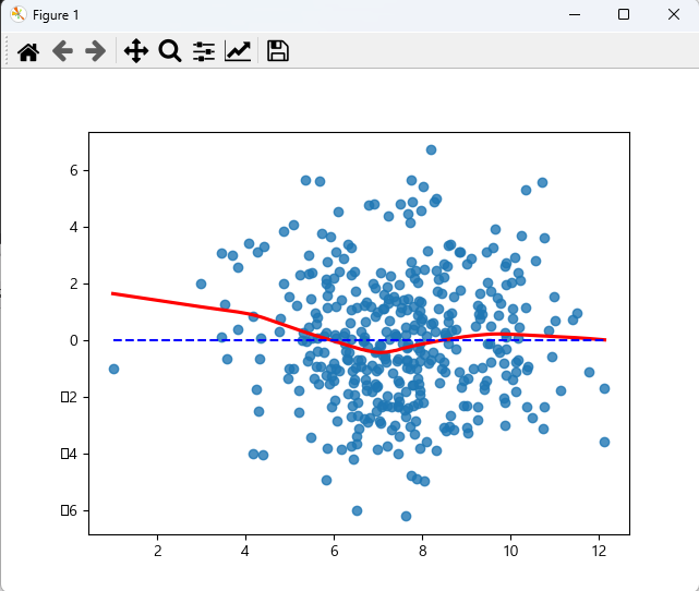
잔차가 일정하게 분포되어 있으므로 선형성 만족
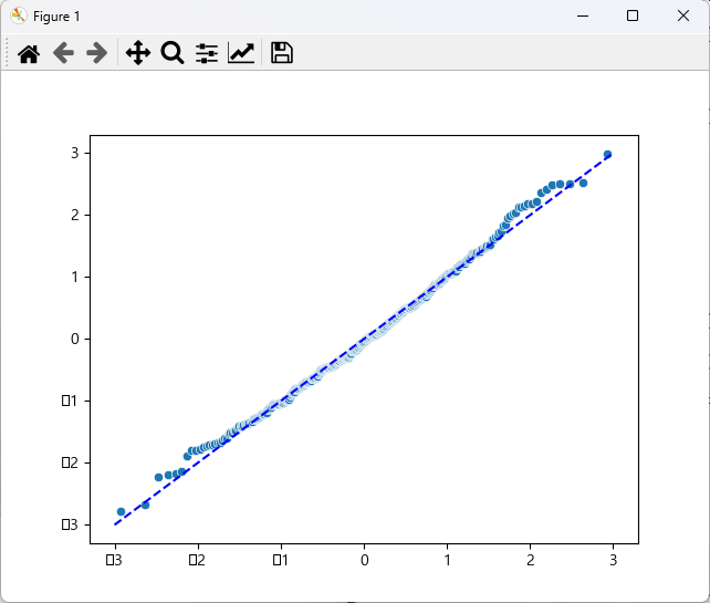
잔차항이 정규분포를 따르므로 정규성 만족

모든 변수가 10을 넘기지 않으므로 다중공선성 우려 없다. 등분산성 만족